Time and Space Complexity

Week 0, day one. Before touching any actual data structure I wanted to get comfortable with the yardstick everything gets measured by: time and space complexity. This is the note I keep coming back to, so I want it solid.

🧠 Classification of Data Structures

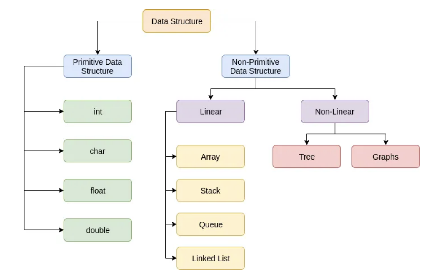
• Data structures split into primitive and non-primitive. Primitives (int, char, float, double) are the basic building blocks that most languages and hardware support directly.
• Non-primitive ones split again into linear and non-linear. Linear structures (arrays, stacks, queues, linked lists) store elements in sequence, which is great for iteration, searching, and anything order-based.
• Non-linear structures (trees and graphs) model messier relationships like file systems, org charts, and web links.
• Knowing this hierarchy actually helps with pattern recognition. A queue for BFS, a tree for recursion-heavy problems, a graph for traversal and connectivity.

🧠 What is time and space complexity?

Time complexity measures how the number of operations grows with the input size n:

• O(1): constant
• O(n): linear
• O(n^2): quadratic
• O(log n): logarithmic

Focus on the dominant term and the worst case. The lower-order stuff washes out for large n.

Space complexity measures how much extra memory you use:

• O(1): constant extra space
• O(n): a hash map or array that scales with input
• O(n): the recursion call stack, which is easy to forget about

📊 Complexity cheat sheet

Complexity	Name	Feasible input size (n)
O(1)	Constant	Instant
O(log n)	Logarithmic	Up to 10^18 and beyond
O(n)	Linear	Up to 10^6 to 10^7
O(n log n)	Linearithmic	Up to 10^5 to 10^6
O(n^2)	Quadratic	Up to 10^3
O(n^3)	Cubic	Up to 100
O(2^n)	Exponential	Up to 20 to 25
O(n!)	Factorial	Up to 10

🎯 Reading the constraints backwards

This is the trick I use most in interviews: the input size basically tells you what complexity the problem is expecting.

• n ≤ 10: O(n!) or O(2^n) is fine, so brute force or backtracking.
• n ≤ 25: O(2^n), think bitmasking and subsets.
• n ≤ 100: O(n^3), triple nested loops are okay.
• n ≤ 1000: O(n^2), often DP.
• n ≤ 1e5: O(n log n) or O(n), so sorting or sliding window.
• n ≤ 1e6 and up: O(n) or O(log n), so hashing or two pointers.

📈 Big-O chart

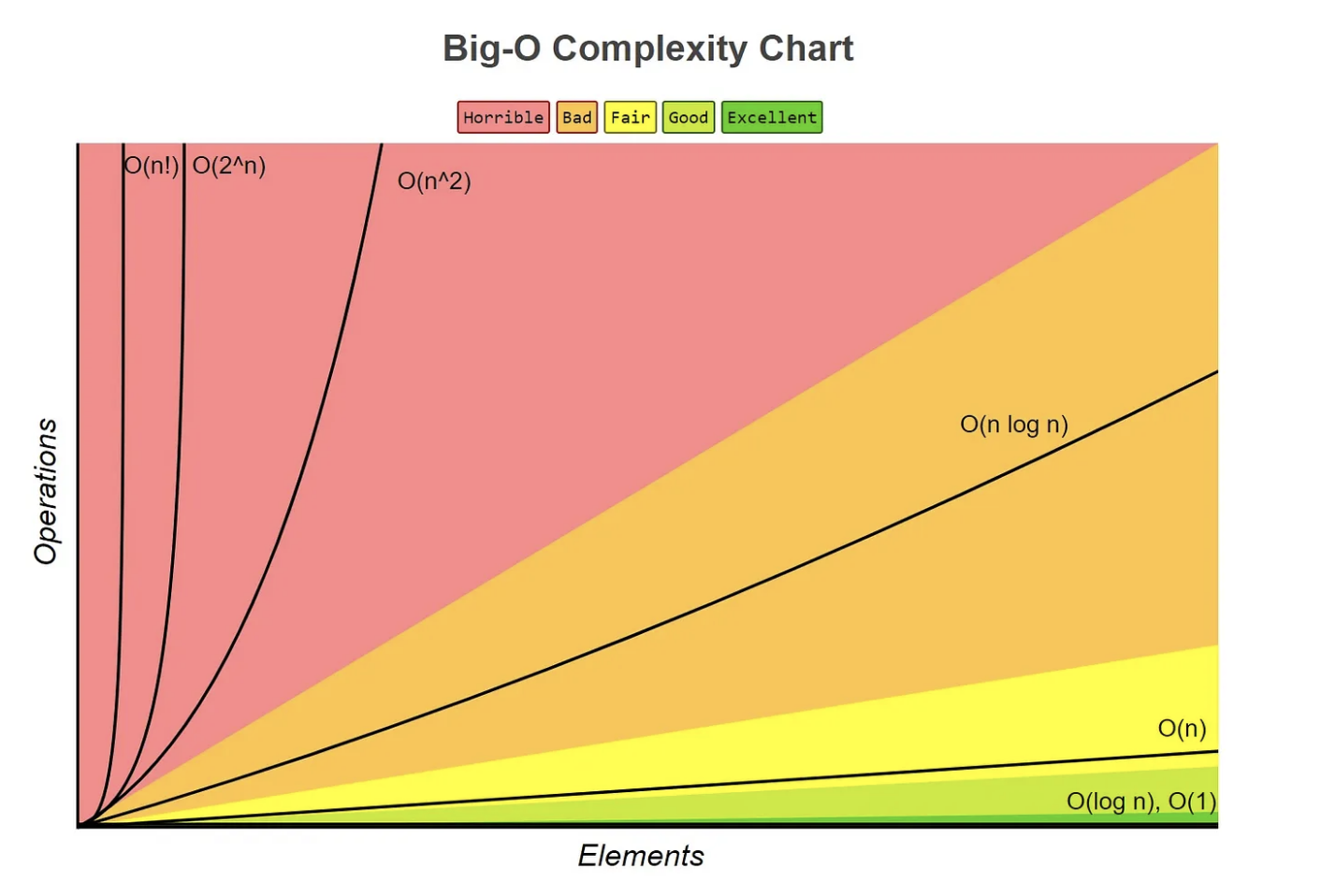
Rough color code I keep in my head:

• Excellent: O(1), O(log n)
• Good to fair: O(n), O(n log n)
• Bad to painful: O(n^2), O(2^n), O(n!)

🌟 A couple of things worth remembering

• Big-O (asymptotic analysis) counts how many operations an algorithm takes, so it lets you compare solutions on efficiency instead of gut feel.
• There’s no single fastest algorithm for everything. It depends on the input and the best/worst-case paths.

If you want to go deeper, this Medium breakdown on Big-O is a good read.

📝 What I want to remember

Analyze the complexity of my approach before I write any code. The constraints usually tell me the target runtime, and building that habit early leads to better instincts and a lot less rewriting.